Chapter 3 Pac-Man Residual Plot

3.1 Description

The results of a regression algorithm typically takes the form of a residual plot, showing the relationship (or lack thereof) between the domain and the residual values of the data associated with the model. From the residual, a broad scope of the model’s performance can be determined.

pacviz contributes a simple approach for looking at the broad view performance of the regression model by constructing a ‘Pac-Man’ residual plot.

3.1.1 Formalism

This visualization technique applies a bijective map from the domain of the data to angular values between 40 and 320 degrees, \[\begin{equation} X: \rightarrow [40, 320]\, . \end{equation}\]

This restriction is applied to allow space for radial labels. By taking the absolute value of the residual values on the radial coordinate system, we can observe the overall performance of the model with relative ease.

In addition, we have added the residual standard deviation for the model both in its numerical form and graphically as a dashed line at one \(\sigma\). This circular segment was created by the circlize package .

There are shortcomings for a visualization that views big-picture components of a model. In the case of the ‘Pac-Man’ residual plot we lose the ability to determine the dependence of the relationship. Through a traditional residual plot, it would be simple to determine if there was systematic or random error based on the relationship between the standard deviation and the domain of the data.

3.2 Usage

The function is setup to implement an arbitrary regression model and supports residual standardization. As we have discussed above,

pac.resid(
  x,y,
  title,
  c(taxislabel, tunits),
  model = lm(y ~ x, data = data.frame(x, y)),
  color1 = "gold",
  standardize = FALSE
)

3.3 Examples

For the following examples, the domain and range that will be processed by the function will be:

data("cars")
x <- cars$dist
y <- cars$speed

The units associated with each of the plots are not accurate, they simply demonstrate the capabilities of the function to use a variety of inputs.

3.3.1 Example 1

In the below snippet, we use

# Generic Pac-Man residual
pac.resid(x,y, 'Example 1',
            c('Axis Label', 'm/s'))

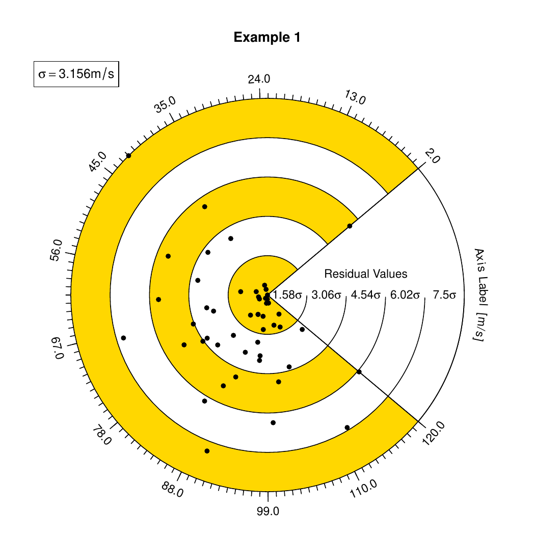
Figure 3.1: Graphical result of Example 1. We can see that the units are attached to the residual standard deviation as well as the angular axis markings. Make note that if you want a space between the numerical value and the units to add a space in the character string.

3.3.2 Example 2

# Pac-Man residual using alternate color,
# residual standardization, and temperature units
pac.resid(x,y, 'Example 2',
            c("Temperature", 'degC'),
            color1="lightblue",
            standardize=TRUE)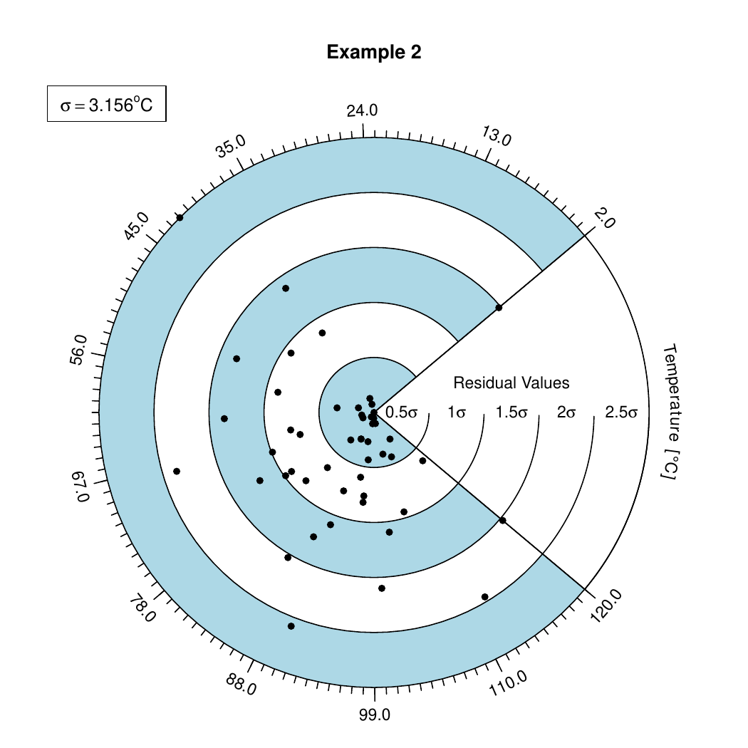

Figure 3.2: Graphical result of Example 2.

3.3.3 Example 3

# Pac-Man residual using alternate color,
# a quadratic model, and a UTF8 character for units
pac.resid(x,y, 'Example 3',
            c("Distance","\uc5"),
            model=lm(y~poly(x,2)),
            color1="darksalmon")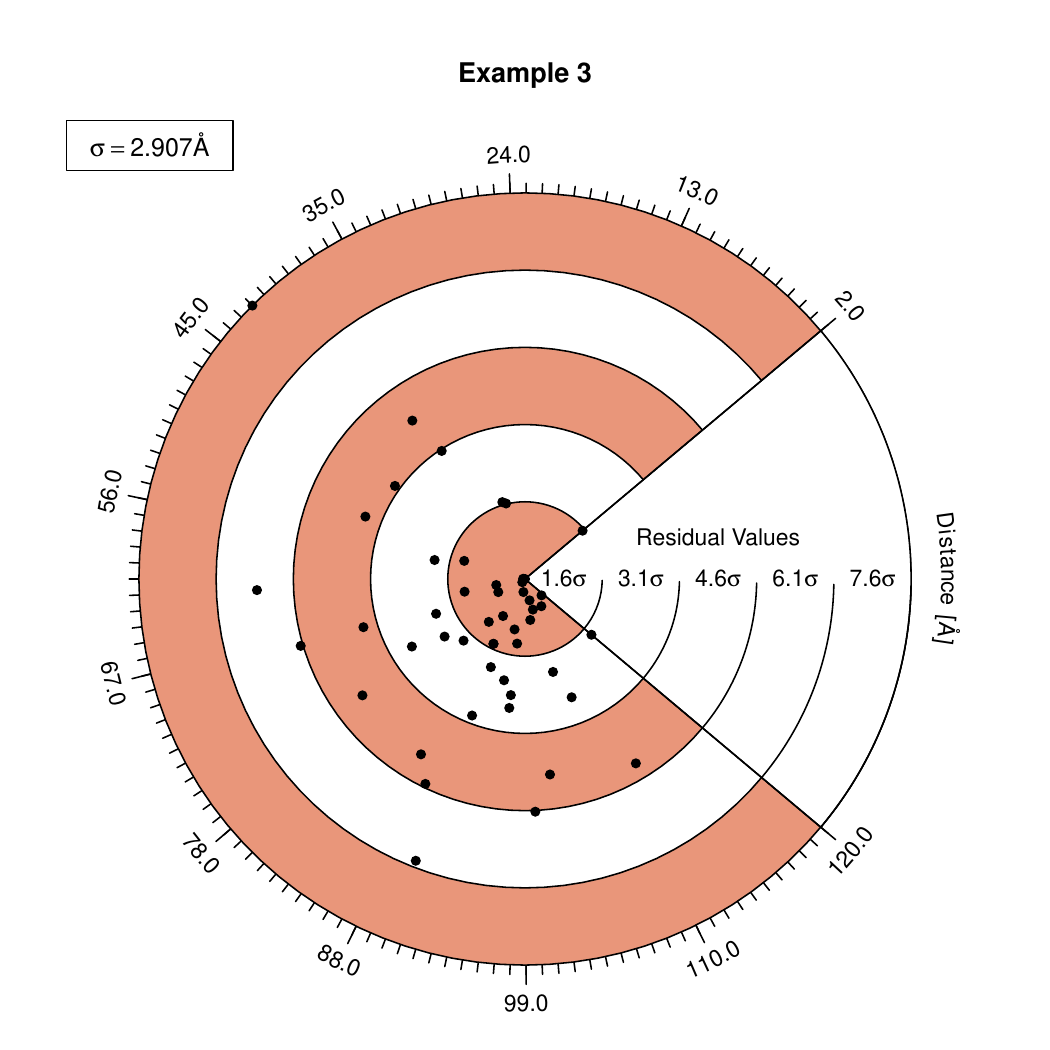

Figure 3.3: Graphical result of Example 3.